What’s the Buzz?
Natural Language Processing (NLP) has become one of the most popular areas in Machine Learning.
A very natural question we can come up with when looking at some text is what is the author talking about. For example we may be interested in providing a recommendation to users on a news site based on their interest in previous articles or to track the buzz around a specific topic in online news.
The goal of Topic Modeling is (unsusprisingly) to identify the topic(s) of a document in order to classify it or provide recommendations.
Latent Dirichlet Allocation (LDA, not to be confused with Fisher’s Linear Discriminant Analysis) is a flexible unsupervised learning tool for clustering documents. First, words are grouped into topics, based on the mutual occurrence within documents in a corpus. Documents are subsequently classified based on the topics they contain. This is called soft clustering: a word can be shared by multiple topics and a document can also be sharing multiple topics.
LDA is at the center of a very florid literature and many methods and extensions have been proposed since the first paper by David Blei. Unfortunately most of them focus on the mathematical or computational details and, in my opinion, neglect the intuition behind the nature of the parameters. In this post I will try to give a simple explanation of the nature of the LDA parameters that goes beyond the notation.
LDA describes the generative model for the words in a corpus of documents, briefly:
- For each document sample the topic distribution \(\theta\sim\)Dirichlet\((\alpha)\)
- For each word \(w_n, n=1,…,N_{d}\) with \(N_d\) number of words in document \(d\):
- sample a topic \(z_n\sim\)Multinomial(\(\theta\) );
- given topic \(z_n\) sample word \(w_n\) from \(p(w_n|z_n,\beta)\).
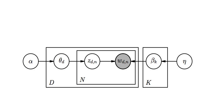
The above graph describes the joint distribution of the variables. The shaded node means that the variable is observed. The only variable we observe are the single words. Everything else is, as the name of the model suggests, Latent.
The quantity of interest in this case is the posterior distribution of the hidden topic variables given the documents, i.e.
\[p(\theta,z|w,\alpha,\beta)=\frac{p(\theta,z,w|\alpha,\beta)}{p(w|\alpha,\beta)}\]in simple words we are interested in the probability of a document being about a topic given that it contains certain words. This is a pretty intuitive concept which is very similar to what a human would do: if an article mentions crops and such, then it’s probably about agriculture, but if such words are in conjunction with terms about trading, then we could conclude that economics is also one of the topics.
Since the direct parameter estimation is intractable, variational inference is typically used. This implies finding a set of lower bounds on the log-likelihood indexed by parameters which will be optimized to get the tightest lower bound possible. This is obtained by slightly modifying the graphical model introducing more parameters.
This is a very common approach, in practice it implies to solve a sequence of simpler problems whose solutions approach the solution to the desired problem.
In the LDA case, for example, we parametrize the topic prior as \(q(\theta,z|\gamma,\phi)=q(\theta|\gamma)\prod_n q(z_n|\phi_n ) \) and smooth over rare words by sampling \(\beta_v\sim\)Dirichlet(\(\lambda_v\)) since ideally we don’t want rare words to have probability zero (a classic Bayesian trick). The resulting graphical model is easier to fit and the optimizing values for the variational parameters can be found minimizing the KL divergence via some simple update equations.
But what do this parameters really represent? What type are those parameters? Let’s look at them one by one and state who they are, what’s their size and support, being \(k=1,…,K\) with \(K\) number of topics and \(v=1,…,V\) with \(V\) number of words. The superscript \(d\) identifies a per-document parameter, while the pedices represent the dimensions of the parameter.
- \(\alpha=\alpha_k\) is the Dirichlet concentration for the topic parameter \(\theta_d\). They are positive valued real numbers. They model how likely is a topic to occur.
- \(z_{d,n}=z^{(d)}_{n,v}\) are the topics of document \(d\), categorical variable distributed multinomially with probabilities \(\theta_{d}\).
- \(\theta_d=\theta^{(d)}_{k}\) is the probability of sampling topic \(k\) from document \(d\). They are probabilities. They represent the confidence of a document being about a certain topic, or the fraction of the document dedicated to a certain topic.
- \(\beta_k=\beta_{k,v}\) are the overall word probabilities conditional on the topic, they are distributed as Dirichlet(\(\lambda_{k,v}\)). They are probabilities. They represent how likely a certain word is to occurr in relation to a certain topic.
The respective variational parameters are:
- \(\gamma^{(d)}_k\) associated to \(\alpha_k\) is the variational parameter for Dirichlet concentration of \(\theta^{(d)}_k\) and is used to compute the expectation of \(\theta^{(d)}_k\). They are positive valued real numbers.
- \(\phi^{(d)}_{k,v}\) associated to \(\theta^{(d)}_k\) is the variational parameter for the topic probabilities. In the variational model they are the expected value of \(z^{(d)}_{n,v}\sim\)Multinom(\(\phi^{(d)}_{k,v}\)). They are probabilities.
- \(\lambda_{v,k}\) is the variational parameter for Dirichlet concentration for \(\beta_{k,v}\) and is used to compute the expectation of \(\beta_{k,v}\). They are positive valued real numbers. This is a crucial parameter associated with the conditional probability of a word belonging to a topic/cluster. Notice how this is an overall parameter and not per-document.